Microsoft Excel Features For The Financially Literate

Microsoft Office Excel is a great computer program that is widely used throughout the financial industry. Microsoft Excel has created incredible efficiencies in the finance and accounting industries. In this article, we'll demonstrate some of Excel's functions and features that a financial professional can use to make his or her job more efficient.

Microsoft Office Excel is a great computer program that is widely used throughout the financial industry. Excel is an invaluable tool for portfolio managers, traders and accountants. Billion dollar portfolios and positions can be managed and traded using Excel spreadsheets. Management reports and risk management tools can be created and run in this program. In short, Microsoft Excel has created incredible efficiencies in the finance and accounting industries. 

In this article, we'll demonstrate some of Excel's functions and features that a financial professional can use to make his or her job more efficient. This article does not discuss Visual Basic for Applications (VBA), but instead focuses on Excel features that non-programmers can deploy. Only basic knowledge of Excel is needed to make use and benefit from this program, so read on to learn about how it can make your job easier.

Inserting Functions

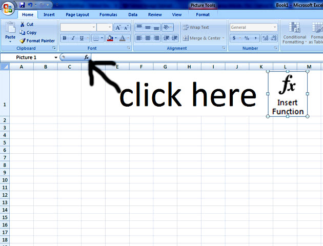
Excel comes with a wide array of functions that can easily be inserted into a spreadsheet. In Microsoft Excel 2010, adding a function is as easy as clicking on the "Insert Function" button from Formulas > Insert Function

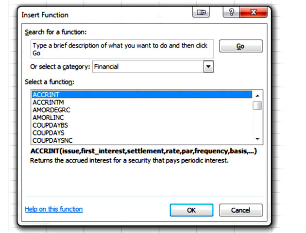
Clicking on the "Insert Function" button allows you to search for a function by typing a brief description of what you want, or by category.

If you click on the "Insert Function" icon, this window will appear:

Adding a particular function to your spreadsheet is then as simple as following the on-screen commands, but if you are ever in doubt, press the F1 key on your keyboard to access Excel's "Help" program.

In addition to financial functions - such as present value, future value, payment and internal rate of return - that are of use to financial professionals, Excel has many functions that are useful in cleaning up and reconciling large data sets, a task frequently encountered by many in finance. Some of these functions are: •

EXACT - Checks whether two strings of text are precisely the same and will return either True or False. •

LEFT, RIGHT or MID - Returns the characters from a text string given a starting position and length, such as the left side, middle of the text string or the right side.

•

TRIM - Will remove, with the exception of single spaces in between different words, all spaces in a text string. •

TRANSPOSE - This function will convert a range of cells aligned vertically to a range of cells aligned horizontally, or vice versa.

The above list is a brief example of just some of the Excel functions. The best way to discover what functions are available and what can be done to make spreadsheets and data manipulation more efficient is simply to play around with Excel's "Insert Function" feature or to take one of Microsoft's courses or tutorials. If you browse by the Text or Lookup & Reference

Look-Up tables

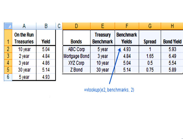
"Look-up" tables are usually a part of any financial spreadsheet or model. In Excel, the "Look-Up" function searches for values in a table based on a certain condition. For example, if you use on-the-run Treasury yields as a benchmark pricing for other bonds, a "Look-Up" table could be used to pull in the appropriate Treasury yield. (To help you learn this function we suggest you open up your own Excel spreadsheet and follow along.) 

In the example above, Column F contains the "Look-Up" formula in each cell, and pulls the appropriate on-the-run Treasury yield from the "Look-Up" table to the left. In this example, the "Look-Up" table runs from Cell A2 to Cell B6. The first value within the "()" of the formula is a cell reference to the value in the "Look-Up" table that is searched for. This means that the value the "Vlookup" function will search for in the "Look-Up" table is a 10-year on-the-run Treasury. The second value in the "Vlookup" function is the name of the "Look-Up" table ("Look-Up" Tables must be named prior to using the "Vlookup" function and are described below). The third value in the "Vlookup" function is the column in the "Look-Up" table that is returned (there can be multiple columns in a "Look-Up" table). 

Creating a "Look-Up" table is a simple, two-step process. 

1. A "Look-Up" table must be sorted in ascending order by the first column. 1.

Using the cursor, highlight the entire data table. 2.

Click on "Data." 3.

Click on "Sort." 

2. You

Looking Up a Value Based on Two Conditions

As demonstrated above, a "Look-Up" table can be used to pull in values based on a certain condition. The user must identify that condition and provide the column in which to find the value that is to be returned. (In the example above, the condition was the name of an on-the-run Treasury bond, and the column was the second column, which contained that particular bond's yield). There is a way to use a "Look-Up" table to return values when the column to be returned is not constant. In other words, based on certain variables, you might want to return the second, third, fourth, etc., columns of a "Look-Up" table. To do this, you must create a "Look-Up" table function within a "Look-Up" table function. 

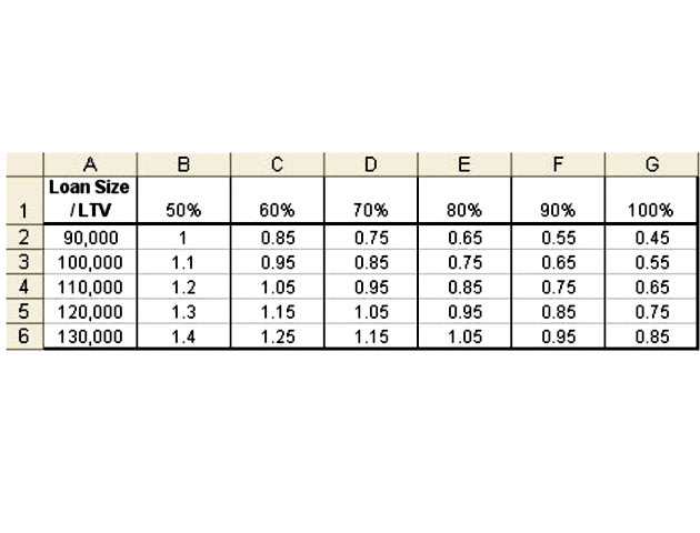
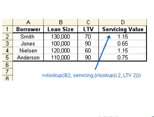
For example, the table below shows the value of mortgage servicing based on loan size and loan-to-value ratios (LTV). Let us call this table the "Servicing Table." 

What if you wanted to pull the value of servicing into a spreadsheet for multiple loans with varying sizes and LTVs? In other words, the column number of the data you want to retrieve is not constant.

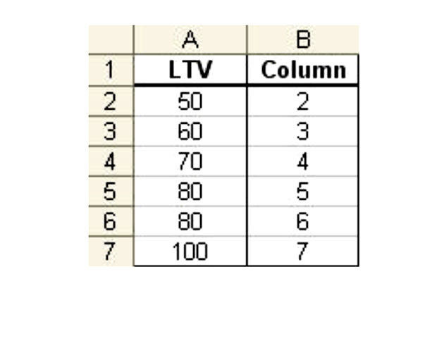
You must first create a separate "Look-Up" table that identifies the column number for a given LTV. Let's create a "Look-Up" table using the following: 

This "Look-Up" table is named "LTV" in the formula shown below. The servicing value "Look-Up" table (the original table in our example) is named "Servicing".

Now you can write a formula to find serving values based on both the variable of loan size and the variable of LTV as shown below.

As you can see from this example, the "Vlookup" function will work when using two different conditions. Keep this information handy, as we will use it in our next section.

The "Exact" Statement

The "Exact" statement (or function) is very useful in working with large sets of data, such as securities, where values within a spreadsheet vary by small amounts (for example, CUSIP numbers). You can use the "Exact" function to ensure that you are pulling in the actual value that you need, or to identify why you might not be able to find a value that you believe should be in the data set.

For example, when using the "Look-Up" function as described above, you must sort the "Look-Up" table by the first column in ascending order. The "Look-Up" function then searches for values in that first column. If a value in the "Look-Up" function cannot be found in the "Look-Up" table, the "Look-Up" function will find the next closest value - this is generally not good in financial spreadsheets, as exact figures are usually required.

For example, if the "Look-Up" function is searching for CUSIP number 912833WZ3, which is not found in the "Look-Up" table, but 912833WZ4 is in the "Look-Up" table, the "Look-Up" function will return the value in the specified column number for the 912833WZ4 CUSIP number. This is simply not the correct CUSIP number.

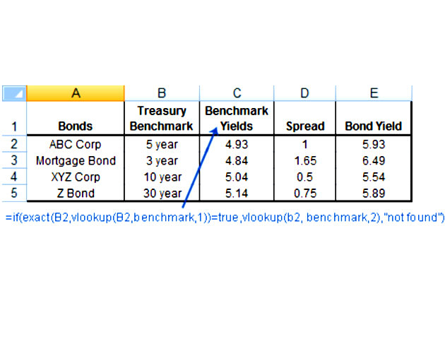
To avoid pulling the closest value when the actual value is not found, use the "Exact" function as shown below.

The "Exact" function shown above says: If the value in Cell B2 is exactly the same as a value found in the "Look-Up" table called "Benchmark," then it will return the value in column two from the table. If

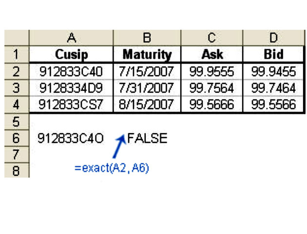
Another common use of the "Exact" function is to figure out why you cannot find a value in a set of data when you "know" it is there. For example, you might be trying to reconcile two sets of data by CUSIP number. You know a certain CUSIP number is in both sets of data, but the formulas you have written aren't recognizing one of the CUSIP numbers as being the same as the other. Simply key the CUSIP number into both spreadsheets, and use the "Exact" function to let Excel tell you whether they are the same - there could be an unseen character in the data, such as a space before the CUSIP number that is causing the problems, which the "Exact" function will help you identify.

As shown above, the "Exact" function is returning a "FALSE." Upon looking closer, the two CUSIPs are different. The CUSIP in A2 ends in "zero" while the CUSIP in A6 ends in "O."

Using Arrays

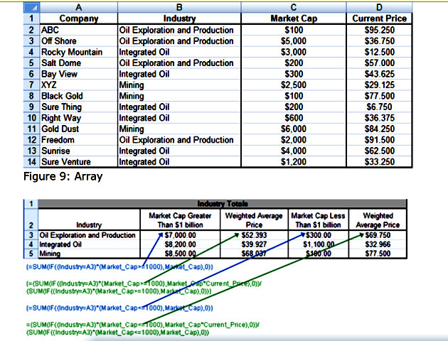
"Arrays" is a powerful feature in Excel that allows you to make calculations within large sets of data based on multiple conditions. For example, using "Arrays," you can sum the value of integrated oil stocks with a certain market cap within a large set of data that consists of stocks from many different industries and with many different market caps, and you can calculate the weighted average price of those stocks. Creating "Arrays" is a simple process, and the first step is to name the "Arrays." 

1. Name the "Arrays." 1.

Using the cursor, highlight the entire set of data, including the column headers (the data must have column headers as they become the names of each "Array"). 2.

Click "Insert" on the tool bar. 3.

Click "Name." 4.

Click "Create." 5.

Mark the "Top Row" check box only and click "OK." 

Writing "Array" functions is also relatively simple. The examples below show "Array" functions that sum the market value of stocks within several industries by market capitalization and calculate the weighted average prices of those stocks based on the data set shown immediately below. 

The "Array" functions are not as complex as they might look at first glance. First, we named the "Arrays" as described above, then we simply use a combination of "If" and "Sum" statements to return values based on the conditions that we set. The weighted average calculation is simply embedded in the "Array" function. The best way to gain expertise using "Arrays" is to